Basics of Decision Trees

Introduction

Decision Trees are a straightforward and interpretable method in Machine Learning. They provide human-like decision-making capabilities to computers and have applications in various fields, from classification tasks like “dog” or “cat” prediction to more complex scenarios like medical diagnoses or customer churn predictions. Understanding Decision Trees can be a great entry point to exploring the vast world of Machine Learning algorithms and their practical uses.

Entropy Intuition

I still remember during my ML class at Georgia Tech, my professors Dr. Charles Isabel and Michael Littman exclaiming at the fact that Claude Shannon invented information theory as part of his Master Thesis; At his Master degree, not even PhD. Its like doing the greatest contribution to this world when you are merely in your Masters. In this section we will try to understand Shannon’s Entropy.

Here is an analogy to understand the intuition behind Entropy.

• Consider the game of “20 Questions” a guesser asks a series of question to find out the name of a celebrity.
• The guesser’s first question is crucial.
• They ask the one that narrows down the options the most.
• Asking specific questions like “Is the celebrity Margot Robbie?” yields no information. If the answer is No, we lost one question with no clue for other 19 questions.
• Asking broader question like “Is the celebrity a woman?” separates the dataset better than specific questions like “Is the celebrity Margot Robbie?”.
• Thus in this example, the “gender” feature has more information than the “name” feature.
• This is the basic intuition that relates to information gain based on entropy.

Entropy Definition

• Shannon’s entropy is defined for a system with N possible states as follows:

\[\Large S = -\sum_{i=1}^{N}p_i \log_2{p_i},\]

where \(p_i\) is the probability of finding the system in the \(i\)-th state.

• This is a very important concept used in physics, information theory, and other areas.
• It helps quantify the level of chaos or disorder in the system.
• If the entropy is high, the system is more disordered, and if it’s low, the system is more ordered.
• This will help us formalize “effective data splitting”, which we alluded to in the context of “20 Questions”.

Entropy Example

Consider a dataset of colored balls with two features: “Position” (numeric value) and “Is Green” (True/False). Our task is to predict whether a ball is green based on its position.

Position	Is Green
0	🟢
1	⚪
2	⚪
3	⚪
4	⚪
5	🟢
6	🟢
7	🟢
8	🟢
9	⚪
10	⚪
11	⚪
12	⚪

We’ll use entropy to guide us in selecting the best position threshold for splitting the data.

1. Entropy of the initial dataset:
   • There are 5 green balls and 8 non-green balls.
   • If we randomly pull out a ball, then it will be green with probability \(p_{g}=\frac{5}{13}\)
   • Similarly at random, we will end up with non-green ball with probability \(p_{ng=}\frac{8}{13}\).
   • Applying \(p_{g}\) and \(p_{ng}\) on the entropy formula, we can arrive at: \(S_0 = -\sum_{i=1}^{2}p_i \log_2{p_i},\) \(S_0 = - (p_{g} \log_2{p_{g}} + p_{ng} \log_2{p_{ng}}),\) \(S_0 = -\frac{5}{13}\log_2{\frac{5}{13}} - \frac{8}{13}\log_2{\frac{8}{13}} \approx 0.96.\)

Entropy of the intial dataset is close to 1.0 which means the intial dataset is highly disordered or chaotic.

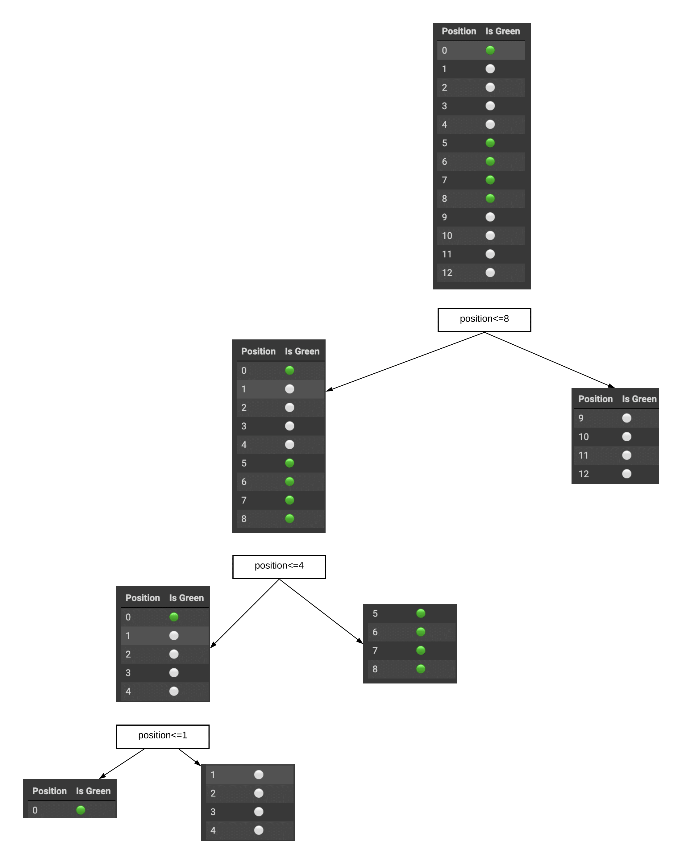
1. Consider splitting the data based on the position threshold “8”:

• Subset1:

Position	Is Green
0	🟢
1	⚪
2	⚪
3	⚪
4	⚪
5	🟢
6	🟢
7	🟢
8	🟢

Lets calculate the entropy for “Position <= 8” (Subset 1):

• \[p_{g=}\frac{5}{9}\]
• \[p_{ng=}\frac{4}{9}\]
• \[S_1 = -\frac{5}{9}\log_2{\frac{5}{9}} - \frac{4}{9}\log_2{\frac{4}{9}} \approx 0.99.\]
• Subset2:

Position	Is Green
9	⚪
10	⚪
11	⚪
12	⚪

Lets calculate the entropy for Entropy for “Position > 8” (Subset 2):

• \[p_{g=}\frac{0}{4}\]
• \[p_{ng=}\frac{4}{4}\]
• \[S_2 = -\frac{0}{4}\log_2{\frac{0}{4}} - \frac{4}{4}\log_2{\frac{4}{4}} = 0.\]

• Therefore, Total Entropy after split on “Position <= 8”: \(S_{\text{Position <= 8}} = \frac{9}{13} \cdot S_1 + \frac{4}{13} \cdot S_2\)

  \[S_{\text{Position <= 8}} = \frac{9}{13} \cdot 0.99 + \frac{4}{13} \cdot 0\] \[S_{\text{Position <= 8}} \approx 0.68.\]

1. As an alternative, lets consider splitting the data based on the position threshold “7”:
   • Entropy for “Position <= 7” (Subset 1):

Position	Is Green
0	🟢
1	⚪
2	⚪
3	⚪
4	⚪
5	🟢
6	🟢
7	🟢

\[S_3 = -\frac{4}{8}\log_2{\frac{4}{8}} - \frac{4}{8}\log_2{\frac{4}{8}} = 1.\]

• Entropy for “Position > 7” (Subset 2):

Position	Is Green
8	🟢
9	⚪
10	⚪
11	⚪
12	⚪

\[S_4 = -\frac{1}{5}\log_2{\frac{1}{5}} - \frac{4}{5}\log_2{\frac{4}{5}} \approx 0.72.\]

• Total Entropy after split on “Position <= 7”: \(S_{\text{Position <= 7}} = \frac{8}{13} \cdot 1 + \frac{5}{13} \cdot 0.72 \approx 0.89.\)

As we can see splitting on position 8 has entropy of 0.68 which is lower than the entropy if split on position 7. Thus we can choose position 8 as our split. We have seen how entropy helps us find the best position threshold for splitting the data and constructing an effective decision tree for predicting the color of a ball based on its position.

Information Gain Definition

Formally, the information gain (IG) for a split based on the variable $Q$ (in this example it’s a variable “$position \leq 8$”) is defined as

\[\Large IG(Q) = S_O - \sum_{i=1}^{q}\frac{N_i}{N}S_i,\]

where $q$ is the number of groups after the split, $N_i$ is number of objects from the sample in which variable $Q$ is equal to the $i$-th value. In our example, our split yielded two groups ($q = 2$), one with 9 elements ($N_1 = 9$), the other with 4 ($N_2 = 4$). Therefore, we can compute the information gain as

\[\Large IG(pos \leq 8) = S_0 - \frac{9}{13}S_1 - \frac{4}{13}S_2 \approx 0.32.\]

It turns out that dividing the balls into two groups by splitting on “position is less than or equal to 8” gave us a more ordered system. If we continue to divide them into groups until the balls in each group are all of the same color, we will end up with a decision tree that predicts ball color based on its position. Note that the entropy of a group where all of the balls are the same color is equal to 0 (\(log_2 1 =0\) ).

Decision Tree Algorithm

The pseudocode provided below can be considered as a high-level overview of the Decision Tree building process. In practice, choosing the best variable to split on (which gives the greatest information gain or minimizes impurity) is a crucial step, and it is typically done using specific metrics like Information Gain for classification tasks or Mean Squared Error reduction for regression tasks.

# Decision Tree Building Algorithm (Classification)

# Function to build the Decision Tree
def build(L):
    create node t

    # Base case: If the stopping criterion is met, assign a predictive model to t (e.g., majority class label for classification)
    if stopping_criterion(L):
        assign_predictive_model(t, L)
    else:
        # Find the best binary split L = L_left + L_right
        L_left, L_right = find_best_split(L)

        # Recursively build the left and right subtrees
        t.left = build(L_left)
        t.right = build(L_right)

    return t

Other Decision Tree heuristics

Gini impurity and misclassification error are other popular heuristics used to evaluate the quality of splits in Decision Trees. While Information Gain and Gini impurity are closely related and often provide similar results, they have different mathematical foundations and properties. The choice of the heuristic can impact the structure and performance of the resulting Decision Tree.

1. Gini Impurity:
   • \[G = 1 - \sum\limits_k (p_k)^2\]
   • Gini impurity is a measure of the impurity or uncertainty of a node in a Decision Tree.
   • It calculates the probability of misclassifying a randomly chosen element from the set if it were randomly classified according to the class distribution of the set.
   • Gini impurity ranges from 0 to 0.5, with 0 representing a pure node (all elements belong to the same class) and 0.5 representing a completely impure node (classes are equally distributed).
   • Gini impurity is often used as an alternative to Information Gain, and the two metrics generally lead to similar splits.

   Lets try calculating the Gini Impurity Values for our Ball Example:

   Subtree	Green vs NG	\(p_g\)	\(p_ng\)	Gini Imp.
   \(S_0\)	🟢-5, ⚪-8	5/13	8/13	0.47
   \(S_1\)	🟢-5, ⚪-4	5/9	4/9	0.49
   \(S_2\)	🟢-0, ⚪-4	0/4	4/4	0.0

   As from our earlier Entropy example, Gini Impurity reduces as the group of balls becomes monochromatic.

2. Misclassification Error:
   • \[E = 1 - \max\limits_k p_k\]
   • Misclassification error, also known as zero-one loss, calculates the proportion of misclassified instances in a node.
   • Unlike Gini impurity and Information Gain, misclassification error is not differentiable, making it less suitable for optimization algorithms.
   • It can be more sensitive to changes in class distribution, especially when dealing with imbalanced datasets, which may lead to suboptimal splits.

In practice, Gini impurity and Information Gain tend to be the more commonly used quality criteria for splitting in Decision Trees. They are both easy to implement, computationally efficient, and can handle multiclass classification problems. Gini impurity is preferred in some libraries (e.g., Scikit-learn) due to its efficiency when dealing with large datasets.

Decision Tree in Regression

When predicting a numeric variable, the idea of a tree construction remains the same, but the quality criteria changes:

• Variance:

\[\Large D = \frac{1}{\ell} \sum\limits_{i =1}^{\ell} (y_i - \frac{1}{\ell} \sum\limits_{j=1}^{\ell} y_j)^2,\]

where \(\ell\) is the number of samples in a leaf, \(y_i\) is the value of the target variable. By finding features that divide the training set in a way that makes the target variable values in each leaf node roughly equal, we can build a tree that predicts numeric values more accurately.

Suppose we have a dataset with a single feature (X) and a target variable (y). Here’s a simplified version of the dataset:

X	y
1	5
2	4
3	7
4	6
5	8

We want to build a decision tree to predict the target variable (y) based on the feature (X). The goal is to find the split point for X that minimizes the total variance in the target variable.

Let’s try different split points for X and calculate the total variance for each split:

1. Split at X <= 2.5:
   • Group 1 (X <= 2.5): y values = [5, 4], mean y = (5 + 4) / 2 = 4.5
   • Group 2 (X > 2.5): y values = [7, 6, 8], mean y = (7 + 6 + 8) / 3 = 7
   • Variance of Group 1 (\(D_1\)) = ((5-4.5)^2 + (4-4.5)^2) / 2 = 0.25
   • Variance of Group 2 (\(D_2\)) = ((7-7)^2 + (6-7)^2 + (8-7)^2) / 3 = 0.67
   • Total Variance (\(D\)) = (0.25 + 0.67) / 5 ≈ 0.18
2. Split at X <= 3.5:
   • Group 1 (X <= 3.5): y values = [5, 4, 7], mean y = (5 + 4 + 7) / 3 = 5.33
   • Group 2 (X > 3.5): y values = [6, 8], mean y = (6 + 8) / 2 = 7
   • Variance of Group 1 (\(D_1\)) = ((5-5.33)^2 + (4-5.33)^2 + (7-5.33)^2) / 3 ≈ 2
   • Variance of Group 2 (\(D_2\)) = ((6-7)^2 + (8-7)^2) / 2 = 0.5
   • Total Variance (\(D\)) = (2 + 0.5) / 5 ≈ 0.5
3. Split at X <= 4.5:
   • Group 1 (X <= 4.5): y values = [5, 4, 7, 6], mean y = (5 + 4 + 7 + 6) / 4 = 5.5
   • Group 2 (X > 4.5): y values = [8], mean y = 8
   • Variance of Group 1 (\(D_1\)) = ((5-5.5)^2 + (4-5.5)^2 + (7-5.5)^2 + (6-5.5)^2) / 4 = 0.625
   • Variance of Group 2 (\(D_2\)) = (8-8)^2 = 0
   • Total Variance (\(D\)) = (0.625 + 0) / 5 ≈ 0.125

Based on the total variance values, we can see that splitting at X <= 4.5 gives the lowest total variance. Therefore, the decision tree will split the data at X <= 4.5 to minimize the variance in the target variable and make more accurate predictions.

MNIST Handwritten Digits Recognition

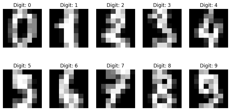
• Recognizing hand written digits is a real world task.
• We will use the sklearn built-in dataset on handwritten digits.
• The images in this dataset are represented as 8x8 matrices, where each element of the matrix represents the intensity of white color for a specific pixel.
• To convert each image into a feature description, we “unfold” the 8x8 matrix into a vector of length 64.
• This vector captures the pixel intensities in a linear sequence, creating a feature representation of the object.

import numpy as np
import matplotlib.pyplot as plt
from sklearn import datasets

# Load the Digits dataset
digits = datasets.load_digits()

# Get the images (data) and target labels
images, data, target_labels = digits.images, digits.data, digits.target


images[0, :]

array([[ 0.,  0.,  5., 13.,  9.,  1.,  0.,  0.],
       [ 0.,  0., 13., 15., 10., 15.,  5.,  0.],
       [ 0.,  3., 15.,  2.,  0., 11.,  8.,  0.],
       [ 0.,  4., 12.,  0.,  0.,  8.,  8.,  0.],
       [ 0.,  5.,  8.,  0.,  0.,  9.,  8.,  0.],
       [ 0.,  4., 11.,  0.,  1., 12.,  7.,  0.],
       [ 0.,  2., 14.,  5., 10., 12.,  0.,  0.],
       [ 0.,  0.,  6., 13., 10.,  0.,  0.,  0.]])

# Visualize some handwritten digits
fig, axes = plt.subplots(2, 5, figsize=(10, 5))
for i, ax in enumerate(axes.flat):
    ax.imshow(images[i], cmap='gray')
    ax.set_title(f'Digit: {target_labels[i]}')
    ax.axis('off')
plt.show()

We will split the dataset into training and holdout sets, with 70% of the data used for training (X_train, y_train) and 30% for holdout (X_holdout, y_holdout). The holdout set will be reserved for final evaluation and will not be involved in tuning the model parameters.

from sklearn.model_selection import train_test_split

X_train, X_holdout, y_train, y_holdout = train_test_split(
    data, target_labels, test_size=0.3, random_state=17
)

We will train a decision tree with random parameters.

from sklearn.tree import DecisionTreeClassifier

tree = DecisionTreeClassifier(max_depth=5, random_state=17)

tree.fit(X_train, y_train)

DecisionTreeClassifier(max_depth=5, random_state=17)

In a Jupyter environment, please rerun this cell to show the HTML representation or trust the notebook.
On GitHub, the HTML representation is unable to render, please try loading this page with nbviewer.org.

We will make predictions on the holdout set.

from sklearn.metrics import accuracy_score

tree_pred = tree.predict(X_holdout)
accuracy_score(
    y_holdout, tree_pred
)

0.6666666666666666

In the process of tuning our model parameters, we will perform cross-validation. However, we have more features, specifically 64, which will impact the complexity of the model and the selection of optimal parameters to achieve better performance.

from sklearn.model_selection import GridSearchCV

tree_params = {
    "max_depth": [1, 2, 3, 5, 10, 20, 25, 30, 40, 50, 64],
    "max_features": [1, 2, 3, 5, 10, 20, 30, 50, 64],
}

tree_grid = GridSearchCV(tree, tree_params, cv=5, n_jobs=-1, verbose=True)

tree_grid.fit(X_train, y_train)

Fitting 5 folds for each of 99 candidates, totalling 495 fits

GridSearchCV(cv=5,
             estimator=DecisionTreeClassifier(max_depth=5, random_state=17),
             n_jobs=-1,
             param_grid={'max_depth': [1, 2, 3, 5, 10, 20, 25, 30, 40, 50, 64],
                         'max_features': [1, 2, 3, 5, 10, 20, 30, 50, 64]},
             verbose=True)

In a Jupyter environment, please rerun this cell to show the HTML representation or trust the notebook.
On GitHub, the HTML representation is unable to render, please try loading this page with nbviewer.org.

listing out the best parameters and the corresponding mean accuracy from cross-validation.

tree_grid.best_params_

{'max_depth': 10, 'max_features': 50}

tree_grid.best_score_

0.8568203376968316

Advantages & Disadvantages

Pros:

1. Generate clear and interpretable classification rules.
2. Easy to visualize both the model and predictions for specific test objects.
3. Fast training and forecasting.
4. Small number of model parameters.
5. Support both numerical and categorical features.

Cons:

1. Sensitivity to noise in input data, which can affect the model’s interpretability.
2. Limitations in separating borders, as decision trees use hyperplanes perpendicular to coordinate axes.
3. Prone to overfitting, requiring pruning or setting constraints on the tree depth and leaf samples.
4. Instability, as small changes to data can significantly alter the decision tree.
5. Difficulty in supporting missing values in the data.
6. Optimal decision tree search is an NP-complete problem, and heuristics are used in practice.
7. The model can only interpolate, not extrapolate, making constant predictions for objects beyond the training data’s feature space.

These limitations should be taken into consideration when using decision trees and can be mitigated through techniques like pruning, ensemble methods, and setting constraints on the tree’s complexity.